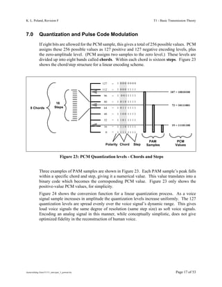
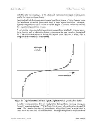
1) The document discusses quantization and pulse code modulation (PCM) in voice signal encoding. PCM assigns 256 possible values to digitally represent analog voice samples, divided into chords and steps on a linear scale.
2) A logarithmic quantization scale is better than a linear one for voice signals, as it allocates more quantization steps to lower amplitudes prevalent in speech. This "compressed encoding" improves fidelity.
3) Quantization error occurs when samples with different amplitudes are assigned the same digital value, distorting the reconstructed waveform. Compression helps maintain a higher signal-to-noise ratio especially for low amplitudes.
The Presentation includes Basics of Non - Uniform Quantization, Companding and different Pulse Code Modulation Techniques. Comparison of Various PCM techniques is done considering various Parameters in Communication Systems.
A Brief Knowledge about Differential Pulse Code Modulation.
It contains the basics of Pulse Code modulation and why we all switching to Differential Pulse Code Modulation.
All the things about the Differential Pulse Code Modulation is given in a good understandable way
introduction to pulse shaping and equalization in advanced digital communication, it's characterisation, signal design of band limited signal, design of bandlimited signal for no ISI and design of bandlimited signal with controlled ISI-partial response, linear equalization,
ATI Courses Satellite Communications Systems Engineering Professional Develop...Jim Jenkins
ATI Courses Satellite Communications Systems Engineering course sampler. This three-day course is designed for satellite communications engineers, spacecraft engineers, and managers who want to obtain an understanding of the "big picture" of satellite communications. Each topic is illustrated by detailed worked numerical examples, using published data for actual satellite communications systems. The course is technically oriented and includes mathematical derivations of the fundamental equations. It will enable the participants to perform their own satellite link budget calculations. The course will especially appeal to those whose objective is to develop quantitative computational skills in addition to obtaining a qualitative familiarity with the basic concepts.
Analog-to-digital conversion is an electronic process in which a continuously variable (analog) signal is changed, without altering its essential content, into a multi-level (digital) signal.
The input to an analog-to-digital converter (ADC) consists of a voltage that varies among a theoretically infinite number of values. Examples are sine waves, the waveforms representing human speech, and the signals from a conventional television camera. The output of the ADC, in contrast, has defined levels or states. The number of states is almost always a power of two -- that is, 2, 4, 8, 16, etc. The simplest digital signals have only two states, and are called binary. All whole numbers can be represented in binary form as strings of ones and zeros.
A general overview of signal encoding
You will learn why to use digital encoding, how signal is transmitted and received and how analog signals are converted to digital
Some digital encoding methods
A presentation prepared by my friend's friend. I have done no editing at all, I'm just uploading the presentation as it is.
Welcome to TechSoup New Member Orientation and Q&A (May 2024).pdfTechSoup
In this webinar you will learn how your organization can access TechSoup's wide variety of product discount and donation programs. From hardware to software, we'll give you a tour of the tools available to help your nonprofit with productivity, collaboration, financial management, donor tracking, security, and more.
Operation “Blue Star” is the only event in the history of Independent India where the state went into war with its own people. Even after about 40 years it is not clear if it was culmination of states anger over people of the region, a political game of power or start of dictatorial chapter in the democratic setup.
The people of Punjab felt alienated from main stream due to denial of their just demands during a long democratic struggle since independence. As it happen all over the word, it led to militant struggle with great loss of lives of military, police and civilian personnel. Killing of Indira Gandhi and massacre of innocent Sikhs in Delhi and other India cities was also associated with this movement.
The Roman Empire A Historical Colossus.pdfkaushalkr1407
The Roman Empire, a vast and enduring power, stands as one of history's most remarkable civilizations, leaving an indelible imprint on the world. It emerged from the Roman Republic, transitioning into an imperial powerhouse under the leadership of Augustus Caesar in 27 BCE. This transformation marked the beginning of an era defined by unprecedented territorial expansion, architectural marvels, and profound cultural influence.
The empire's roots lie in the city of Rome, founded, according to legend, by Romulus in 753 BCE. Over centuries, Rome evolved from a small settlement to a formidable republic, characterized by a complex political system with elected officials and checks on power. However, internal strife, class conflicts, and military ambitions paved the way for the end of the Republic. Julius Caesar’s dictatorship and subsequent assassination in 44 BCE created a power vacuum, leading to a civil war. Octavian, later Augustus, emerged victorious, heralding the Roman Empire’s birth.
Under Augustus, the empire experienced the Pax Romana, a 200-year period of relative peace and stability. Augustus reformed the military, established efficient administrative systems, and initiated grand construction projects. The empire's borders expanded, encompassing territories from Britain to Egypt and from Spain to the Euphrates. Roman legions, renowned for their discipline and engineering prowess, secured and maintained these vast territories, building roads, fortifications, and cities that facilitated control and integration.
The Roman Empire’s society was hierarchical, with a rigid class system. At the top were the patricians, wealthy elites who held significant political power. Below them were the plebeians, free citizens with limited political influence, and the vast numbers of slaves who formed the backbone of the economy. The family unit was central, governed by the paterfamilias, the male head who held absolute authority.
Culturally, the Romans were eclectic, absorbing and adapting elements from the civilizations they encountered, particularly the Greeks. Roman art, literature, and philosophy reflected this synthesis, creating a rich cultural tapestry. Latin, the Roman language, became the lingua franca of the Western world, influencing numerous modern languages.
Roman architecture and engineering achievements were monumental. They perfected the arch, vault, and dome, constructing enduring structures like the Colosseum, Pantheon, and aqueducts. These engineering marvels not only showcased Roman ingenuity but also served practical purposes, from public entertainment to water supply.
Macroeconomics- Movie Location
This will be used as part of your Personal Professional Portfolio once graded.
Objective:
Prepare a presentation or a paper using research, basic comparative analysis, data organization and application of economic information. You will make an informed assessment of an economic climate outside of the United States to accomplish an entertainment industry objective.
How to Make a Field invisible in Odoo 17Celine George
It is possible to hide or invisible some fields in odoo. Commonly using “invisible” attribute in the field definition to invisible the fields. This slide will show how to make a field invisible in odoo 17.
Honest Reviews of Tim Han LMA Course Program.pptxtimhan337
Personal development courses are widely available today, with each one promising life-changing outcomes. Tim Han’s Life Mastery Achievers (LMA) Course has drawn a lot of interest. In addition to offering my frank assessment of Success Insider’s LMA Course, this piece examines the course’s effects via a variety of Tim Han LMA course reviews and Success Insider comments.
2024.06.01 Introducing a competency framework for languag learning materials ...Sandy Millin
http://sandymillin.wordpress.com/iateflwebinar2024
Published classroom materials form the basis of syllabuses, drive teacher professional development, and have a potentially huge influence on learners, teachers and education systems. All teachers also create their own materials, whether a few sentences on a blackboard, a highly-structured fully-realised online course, or anything in between. Despite this, the knowledge and skills needed to create effective language learning materials are rarely part of teacher training, and are mostly learnt by trial and error.
Knowledge and skills frameworks, generally called competency frameworks, for ELT teachers, trainers and managers have existed for a few years now. However, until I created one for my MA dissertation, there wasn’t one drawing together what we need to know and do to be able to effectively produce language learning materials.
This webinar will introduce you to my framework, highlighting the key competencies I identified from my research. It will also show how anybody involved in language teaching (any language, not just English!), teacher training, managing schools or developing language learning materials can benefit from using the framework.
Instructions for Submissions thorugh G- Classroom.pptxJheel Barad
This presentation provides a briefing on how to upload submissions and documents in Google Classroom. It was prepared as part of an orientation for new Sainik School in-service teacher trainees. As a training officer, my goal is to ensure that you are comfortable and proficient with this essential tool for managing assignments and fostering student engagement.
Model Attribute Check Company Auto PropertyCeline George
In Odoo, the multi-company feature allows you to manage multiple companies within a single Odoo database instance. Each company can have its own configurations while still sharing common resources such as products, customers, and suppliers.
1. K. L. Poland, Revision F T1 - Basic Transmission Theory
7.0 Quantization and Pulse Code Modulation
If eight bits are allowed for the PCM sample, this gives a total of 256 possible values. PCM
assigns these 256 possible values as 127 positive and 127 negative encoding levels, plus
the zero-amplitude level. (PCM assigns two samples to the zero level.) These levels are
divided up into eight bands called chords. Within each chord is sixteen steps. Figure 23
shows the chord/step structure for a linear encoding scheme.
127 = 1 000 0000
112 = 1 000 1111
107 = 10010100
96 = 1 0011111
80 = 1 010 1111
16
72 = 10111001
8 Chords Steps 64 = 1 011 1111
48 = 1 100 1111
32 = 1 101 1111
16 = 1 110 1111 19 = 11101100
0 = 1 111 1111
PAM PCM
Polarity Chord Step Samples Values
Figure 23: PCM Quantization levels - Chords and Steps
Three examples of PAM samples are shown in Figure 23. Each PAM sample’s peak falls
within a specific chord and step, giving it a numerical value. This value translates into a
binary code which becomes the corresponding PCM value. Figure 23 only shows the
positive-value PCM values, for simplicity.
Figure 24 shows the conversion function for a linear quantization process. As a voice
signal sample increases in amplitude the quantization levels increase uniformly. The 127
quantization levels are spread evenly over the voice signal’s dynamic range. This gives
loud voice signals the same degree of resolution (same step size) as soft voice signals.
Encoding an analog signal in this manner, while conceptually simplistic, does not give
optimized fidelity in the reconstruction of human voice.
/home/tellabg-2/ken/T1/T1_intro/part_3_portrait.fm Page 17 of 53
2. T1 - Basic Transmission Theory K. L. Poland, Revision F
Voice signal
amplitude
Quantization value
Figure 24: Linear Quantization, Signal Amplitude versus Quantization Value
Notice this transfer function gives two values for a zero-amplitude signal. In PCM, there
is a “positive zero” and a “negative zero”.
7.1 Companding
Dividing the amplitude of the voice signal up into equal positive and negative steps is not
an efficient way to encode voice into PCM. Figure 23 shows PCM chords and steps as
uniform increments (such as would be created by the transfer function depicted in Figure
24). This does not take advantage of a natural property of human voice: voices create low-
amplitude signals most of the time (people seldom shout on the telephone). That is, most
of the energy in human voice is concentrated in the lower end of voice’s dynamic range.
To create the highest-fidelity voice reproduction from PCM, the quantization process must
take into account this fact that most voice signals are typically of lower amplitude. To do
this the vocoder adjusts the chords and steps so that most of them are in the low-amplitude
Page 18 of 53 /home/tellabg-2/ken/T1/T1_intro/part_3_portrait.fm
3. K. L. Poland, Revision F T1 - Basic Transmission Theory
end of the total encoding range. In this scheme, all step sizes are not equal. Step sizes are
smaller for lower-amplitude signals.
Quantization levels distributed according to a logarithmic, instead of linear, function gives
finer resolution, or smaller quantization steps, at lower signal amplitudes. Therefore,
higher-fidelity reproduction of voice is achieved. Figure 25 shows a conversion function
for a logarithmic quantization process.
A vocoder that places most of the quantization steps at lower amplitudes by using a non-
linear function, such as a logarithm, is said to compress voice upon encoding, then expand
the PCM samples to re-create an analog voice signal. Such a vocoder is hence called a
compander (from compress and expand).
Voice signal
amplitude
Quantization value
Figure 25: Logarithmic Quantization, Signal Amplitude versus Quantization Value
In reality, voice quantization does not exactly follow the logarithmic curve step for step, as
Figure 25 appears to indicate. PCM in North America uses a logarithmic function called
µ-law. The encoding function only approximates a logarithmic curve, as steps within a
chord are all the same size, and therefore linear. The steps change in size only from chord
/home/tellabg-2/ken/T1/T1_intro/part_3_portrait.fm Page 19 of 53
4. T1 - Basic Transmission Theory K. L. Poland, Revision F
to chord. The chords form linear segments that approximate the µ-law logarithmic curve.
The chords form a piece-wise linear approximation of the logarithmic curve.
7.2 Quantization Error
Figure 26 shows three PAM samples that have their amplitudes measured and given PCM
values. If a PAM sample’s level lies between two steps, it is assigned the value of the
highest step it crosses. A PAM sample that just reaches this step would be given the same
quantization value. Therefore, all PAM samples are treated as if they fall exactly on a step
level.
PAM samples with amplitudes that are not close to each other (e.g., B & C in Figure 26)
can be given the same quantization value. Even though the PAM samples represent
different amplitudes of the original signal, they receive the same PCM value. This causes
an impreciseness in the voice encoding process called quantization error.
Figure 26 shows how the quantization process can alter a voice signal. Samples A and B
are closest in amplitude, with C being much lower. However, due to how the samples fall
into the quantization levels, the sample steps created from the PCM words have B and C at
the same amplitude. Obviously, the reconstructed waveform will be different from the
original waveform.
Sample A
Sample B
Sample C
one step
Quantization level steps Encode: PAM to PCM Decode: PCM to Step
Figure 26: Quantization Error: Recovered Step levels do not match PAM levels
7.2.1 Fidelity: Maintaining a high Signal-to-Noise ratio
Quantization error is another reason for using compressed encoding for digitizing a voice
signal. Compressed encoding allows a higher signal-to-quantization-noise ratio (SNQR)
than linear encoding. This ratio defined as
S
SN Q R = 20log 〈 -------〉
NQ
Page 20 of 53 /home/tellabg-2/ken/T1/T1_intro/part_3_portrait.fm
5. K. L. Poland, Revision F T1 - Basic Transmission Theory
where S is the voice signal level and NQ is noise due to the quantization error. Clearly,
keeping the quantization error small is key to keeping a high SNQR. As signal amplitude
gets smaller, NQ must get smaller to keep SNQR from dropping. Compression
accomplishes this by forcing quantization error magnitude to decrease with lower
amplitudes.
Step
Higher amplitude
Waveform to quantize
Chord
Magnification of small signal
Lower amplitude
PAM sample
Figure 27: Linear Quantization, another View
Without increasing the overall number of quantization samples, it is desirable to increase
the SNQR for small-amplitude signals. This is what logarithmic quantization
accomplishes.
Figure 27 gives another view (as opposed to Figure 24) of the scale for a linear quantizer.
The quantization levels are shown to the left for the positive range of a voice waveform.
This is only the positive half of the quantization scale. There is a mirror image scale for
/home/tellabg-2/ken/T1/T1_intro/part_3_portrait.fm Page 21 of 53
6. T1 - Basic Transmission Theory K. L. Poland, Revision F
the negative half of the voice signal (not shown here for simplicity). The magnification of
a small-amplitude portion of the voice signal shows the relative coarseness of the sampling
function. Few sample levels for a small signal corresponds to a low-fidelity (low SNQR)
encoding technique.
Step
Higher amplitude
Waveform to quantize
Chord
Magnification of small signal
Lower amplitude
PAM sample
Figure 28: Logarithmic Quantization, another View
Figure 28 gives another view (as opposed to Figure 25) of a logarithmic quantizer process.
The magnification of a low-amplitude region of the signal shows how sampling levels are
close together, compared to the same low-amplitude signal quantized by linear encoding
(see Figure 27). Smaller quantizing steps for low-amplitude signals allows a better signal-
to-noise ratio, which amounts to better fidelity, when sampling voice signals.
Page 22 of 53 /home/tellabg-2/ken/T1/T1_intro/part_3_portrait.fm